Warren Buffett famously used to buy his breakfast at the same McDonald’s in Omaha on his way to work. Forbes puts his net worth at about $148 billion.
Imagine he walks in one morning and joins 49 other people having breakfast. Say each of them has the net worth of a typical American household, about $193,000 (the Federal Reserve’s most recent survey).
What’s the average net worth of the people in that McDonald’s?
- The average is about $3 billion. On average, everyone in the restaurant is a billionaire.
- The median is still $193,000. Half the people have more, half have less, and Buffett walking in doesn’t change that at all.
The average isn’t wrong, exactly. It’s a correct calculation that describes nobody in the room.
And if you tried to draw this as a histogram, with each $200,000 range as a bar 1 cm wide, the 49 regular customers would all be in the first bar. Buffett’s bar would be about 7.4 kilometres to the right.
So far, so familiar: outliers break averages, so use the median. But I wanted to see what this looks like with real latency data. It turns out the median isn’t the end of the story either.
the data Link to heading
I’ve been measuring how long this blog takes to load using probe, a small Go tool I wrote that sends the same request over and over and times each one. Everything here comes from my laptop in Kerala, over Wi-Fi, talking to Cloudflare in Chennai.
Here are 1,001 requests, each on a fresh connection:
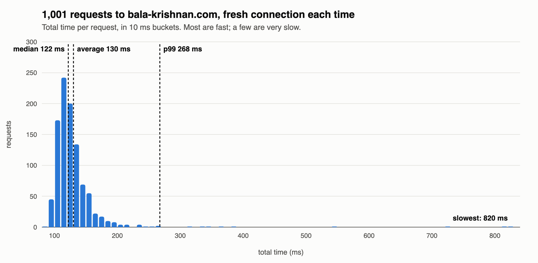
Most requests take between 100 and 150ms. Then there’s a long, thin tail: a handful of requests out at 300, 500, 700 and 820ms.
- average: 130ms
- median: 122ms
- p99: 268ms (99% of requests were faster than this)
This is the Buffett effect on a small scale. The slow requests drag the average above the median, though not by much, because there are only a few of them. If you only looked at the average, you’d say “about 130ms” and that would be… fine?
Here’s where it stops being fine.
the average says nothing changed Link to heading
Those 1,001 requests came from five separate runs of 200, on different days and at different times. Here’s the average and the p99 for each run:
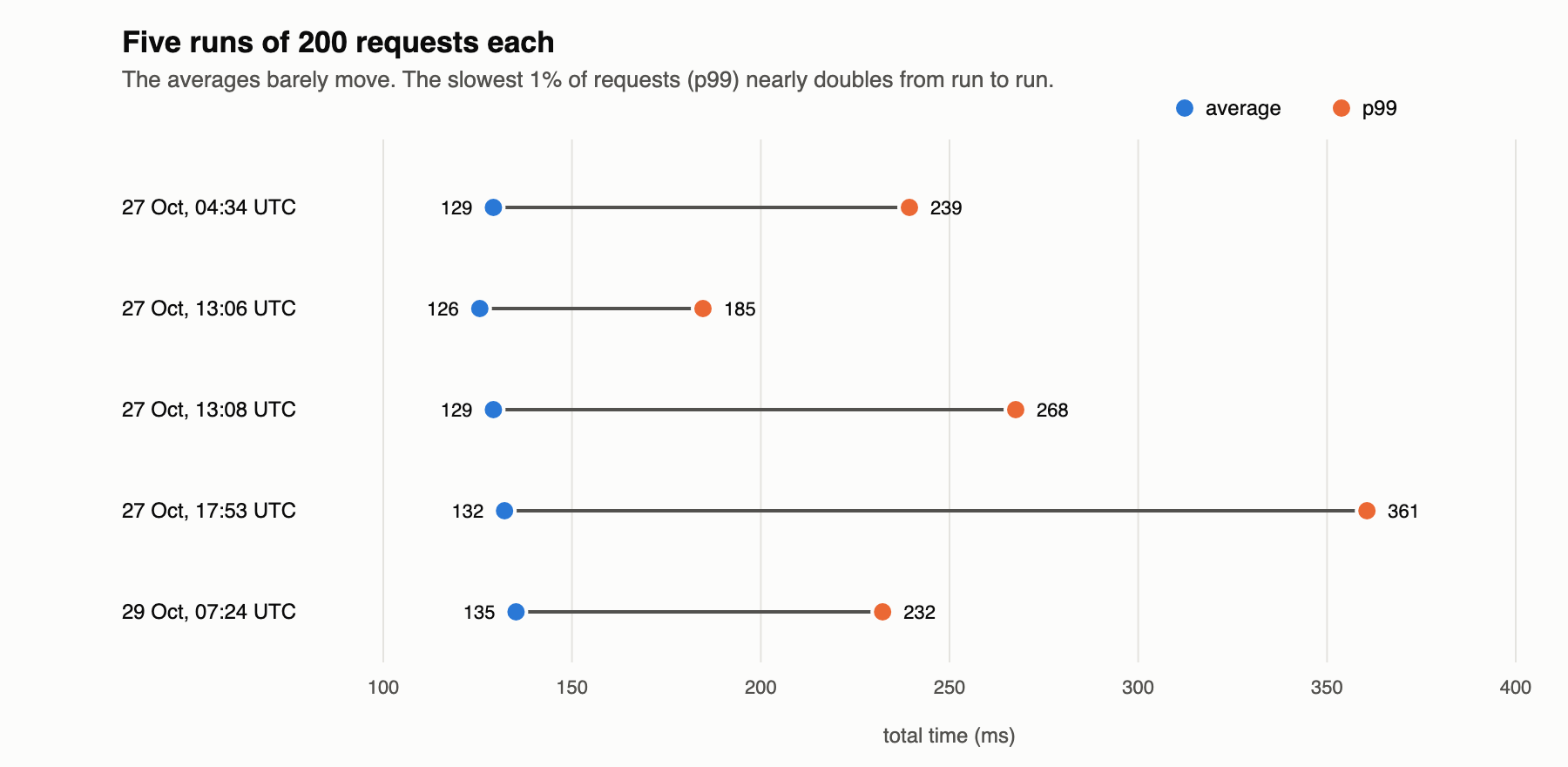
The five averages are all within 10ms of each other: 126 to 135ms. If you were watching an average, you’d conclude the site behaved exactly the same every time.
The p99s range from 185ms to 361ms. The slowest 1% of requests in the 17:53 run were about twice as slow as the slowest 1% in the 13:06 run. Something was different about that run (probably my Wi-Fi), and the average didn’t notice.
This is the version that matters for SREs. The people having a bad time are in the tail, and the average is the number that’s least sensitive to the tail.
what a dashboard would have shown Link to heading
Most latency dashboards don’t plot every request. They plot one point per time window, often an average. Here’s that 17:53 run, with every request as a dot and the line a dashboard would draw:
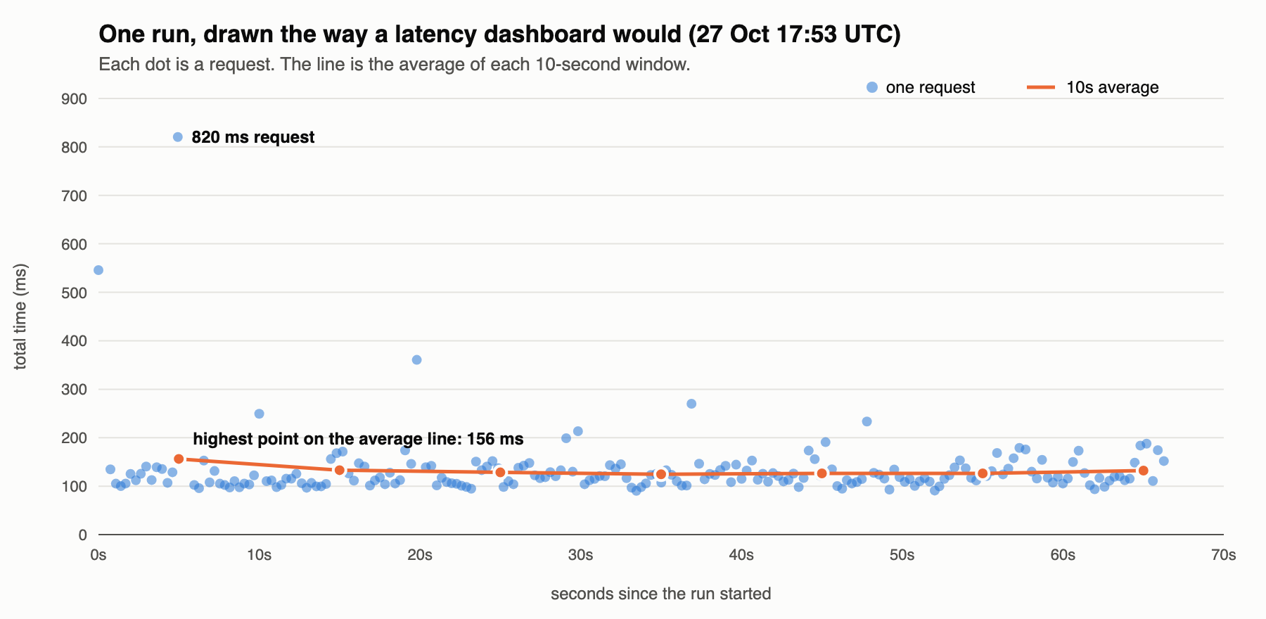
One request took 820ms. The highest point on the average line is 156ms.
If you’d set an alert for “average latency above 300ms”, it would never have fired. Someone waited most of a second, and the graph stayed flat.
the median fails too Link to heading
So far, the advice is the usual one: use the median and the percentiles, not the average. But here’s an experiment that breaks the median as well.
probe can either open a fresh connection for every request (like a first-time visitor) or reuse one connection (like a reader clicking around the site). On 29 October I did one run of each, back to back. Here are all 400 requests together:
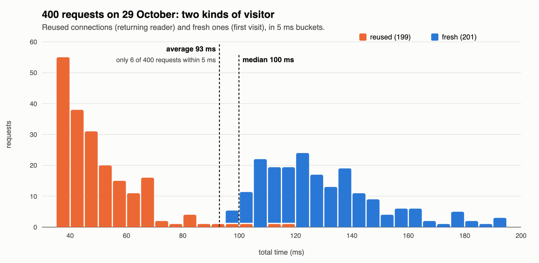
There are two humps, because there are two kinds of request:
- reused connections take about 45ms
- fresh connections take about 120ms, because they have to do the DNS lookup and the TCP and TLS handshakes first
Now look at the two lines:
- The average is 93ms, right in the empty gap between the humps. Only 6 of the 400 requests were within 5ms of it. Like the billionaire breakfast crowd, it describes a request that almost never happened.
- The median is 100ms, at the bottom edge of the fresh hump. It isn’t a typical fresh request, and it’s nowhere near a typical reused one.
This is the bit I didn’t expect. With two groups mixed together, no single number describes either of them. The median survives an outlier, but it can’t tell you there are two different populations. Only the histogram shows that.
so, why histograms? Link to heading
An average gives you one number. A median and a few percentiles give you a handful. A histogram gives you the shape, and the shape is where the interesting things are:
- A long tail means some users are having a much worse time than the typical one.
- Two humps mean you’re looking at two different things mixed together: cache hits and misses, fresh and reused connections, two regions, two versions of a deploy. The fix is to split them and look at each one.
- A cluster far from the main hump usually has one specific cause. In my probe post, a cluster at about 1.1 seconds turned out to be lost packets being retried after exactly one second.
I find it reassuring that Prometheus agrees: its latency metrics are literally histograms (_bucket series), and histogram_quantile() works out percentiles from the bucket counts. If you’ve written a latency SLO, there’s a histogram underneath it. I wrote more about the statistics behind alerts a while ago.
things I’m still not sure about Link to heading
- How should you pick bucket sizes? In the two-humps chart, 5ms buckets show the gap clearly. With 50ms buckets the gap disappears. I don’t know a good rule for choosing them, beyond trying a few.
- When is the average actually the right number? For capacity planning, total work done over time is what matters, and that’s an average times a count. I think “averages are always bad” is too strong, but I haven’t worked out exactly where the line is.
probe is on my GitHub if you want to run the same experiment against your own site.